How to Remove Duplicates in Google Sheets

A customer gets entered twice. Someone submits the same form more than once. Two exports get combined and bring the same records with them. Before long, counts are off, mailing lists are messy, and reports don’t quite add up.

If you’re trying to remove duplicates Google Sheets data, you’ve got several options. The quickest is Google’s built-in Remove duplicates tool. But deleting rows isn’t always the smartest move.

Sometimes you need to see the duplicates first. Sometimes you want a clean list without touching the original data. And sometimes two entries only look identical because an extra space is hiding in one of them.

Google Sheets gives you tools for all of those situations. The trick is knowing which one to use.

What Does Google Sheets Count as a Duplicate?

Before deleting anything, decide what “duplicate” actually means in your sheet.

It sounds obvious, but this is where many cleanup mistakes start.

Imagine this customer list:

Name	Email	City
Sarah Lee	[email protected]	Austin
Sarah Lee	[email protected]	Austin
Sarah Lee	[email protected]	Dallas

If you compare all three columns, only the first two rows match.

If you compare only the Email column, all three rows share the same value.

That’s a big difference.

Duplicate Check	What Gets Compared	Good For
One column	One identifying field	Emails, SKUs, IDs
Several columns	A combination of fields	Orders, registrations
Full row	Every selected field	Fully repeated records
Formula-based list	Rules you define	Reports and live cleanup

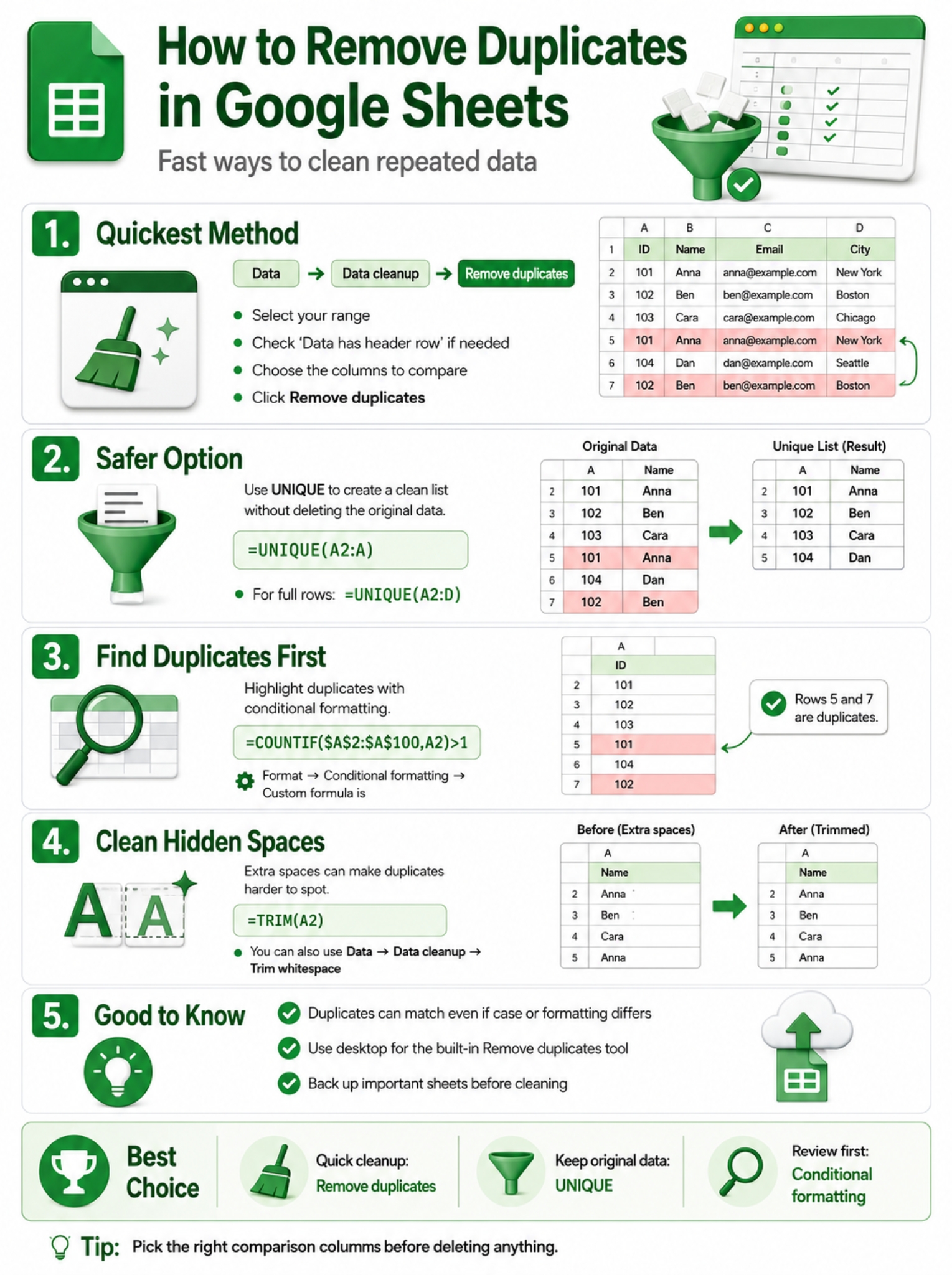
Google’s built-in tool lets you choose which columns count toward the comparison.

There’s another detail worth knowing. Google says values can count as duplicates even when their capitalization, formatting, or formulas differ, as long as the resulting values match.

That means two cells showing the same value may be treated as duplicates even if one comes from a formula and the other was typed manually.

So don’t assume that visual differences will protect a row from being removed.

Remove Duplicates Google Sheets With the Built-In Tool

For a quick one-time cleanup, this is the easiest method.

On a computer:

1. Open your spreadsheet.
2. Select the range you want to clean.
3. Click Data.
4. Choose Data cleanup.
5. Click Remove duplicates.
6. Select Data has header row if your range includes headings.
7. Choose the columns Sheets should compare.
8. Click Remove duplicates.

Google Sheets will remove matching records from the selected range and tell you how many rows it removed.

Step	What to Watch
Select the range	Include all related columns
Mark the header	Prevent headings from being treated as data
Pick comparison columns	Decide what makes a row duplicate
Remove duplicates	Review the setup before confirming

The column choice is the part that deserves the most attention.

Say your sheet contains:

• Customer ID
• Email
• Purchase date
• Product
• Amount

If you tell Sheets to compare only the Email column, every repeated email may count as a duplicate.

That’s fine for a newsletter list.

It’s a bad idea for an order history where one customer may have made ten different purchases.

Before you click the final button, ask one simple question:

What field actually makes this record unique?

Remove Duplicates Based on One Column or Several Columns

Google Sheets doesn’t force you to compare every column.

You can decide which fields matter.

Type of Data	Useful Comparison Field
Newsletter list	Email address
Inventory	SKU
Employee database	Employee ID
Event registrations	Email + event name
Sales records	Order ID
Survey data	Response ID

Example: Clean a Repeated Email List

Suppose your table looks like this:

Name | Email | Company | City

If your only goal is one row per email address, select the whole table but use Email as the comparison column.

That way, Sheets checks the email while keeping the other fields tied to each row.

Example: Compare Two Fields

Now imagine you manage event registrations.

The same person may attend more than one event, so using Email alone would be too broad.

Instead, compare:

Email + Event Name

That combination lets the same person appear at different events without being treated as a duplicate.

This is why duplicate cleanup isn’t just about spotting repeated text. It’s about defining a unique record correctly.

Use UNIQUE When You Don’t Want to Delete Anything

Sometimes deleting rows feels too risky.

That’s where UNIQUE comes in.

Instead of removing anything from your source data, the function creates a separate list containing distinct values or rows.

Google documents the syntax as:

UNIQUE(range, by_column, exactly_once)

For a basic list:

=UNIQUE(A2:A)

For full rows across several columns:

=UNIQUE(A2:D)

Formula	What It Does
=UNIQUE(A2:A)	Returns distinct values
=UNIQUE(A2:D)	Returns distinct rows
=UNIQUE(FILTER(A2:A,A2:A<>””))	Removes blanks from the result
=UNIQUE(A2:A,FALSE,TRUE)	Returns values that appear only once

The source stays where it is.

That’s useful when you’re building:

• contact lists;
• reporting tables;
• dashboards;
• campaign audiences;
• product lists;
• dropdown sources.

For example, if column B contains email addresses, enter:

=UNIQUE(B2:B)

You get a clean list without deleting a single record from the original column.

Remove Blank Results Too

If the source contains empty cells, try:

=UNIQUE(FILTER(A2:A,A2:A<>””))

FILTER removes blank entries first, then UNIQUE removes repeated values.

Return Only Values That Appear Once

There’s also a less-known option:

=UNIQUE(A2:A,FALSE,TRUE)

The last argument tells Sheets to return only values that occur exactly once.

That’s not the same as normal deduplication.

If Apple appears three times, normal UNIQUE returns Apple once.

With exactly_once set to TRUE, Apple won’t appear at all.

This can help when you’re looking for one-off IDs, unmatched records, or unusual responses.

Highlight Duplicates Before Deleting Them

Deleting duplicates immediately isn’t always the best move.

If the data matters, highlight the repeats first.

Google Sheets can do this with conditional formatting.

Suppose your list runs from A2:A100.

1. Select A2:A100.
2. Click Format.
3. Choose Conditional formatting.
4. Under the rule type, choose Custom formula is.
5. Enter:

=COUNTIF($A$2:$A$100,A2)>1

1. Choose a formatting style.
2. Click Done.

Every repeated value in the range will now stand out visually.

Method	Deletes Data?	Best Use
Remove duplicates	Yes	Quick permanent cleanup
Conditional formatting	No	Review before deleting
UNIQUE	No	Create a separate clean list
Manual review	No	Sensitive records

This is especially useful when repeated values don’t mean repeated records.

Two customers may share a company phone number. Two orders may use the same email. Two employees may have the same name.

Highlighting gives you a chance to see what’s really happening before you remove anything.

Read Also: How to Merge Cells in Excel Without Losing Data

Clean Extra Spaces Before Removing Duplicates

One of the most annoying spreadsheet problems is the duplicate that doesn’t look like a duplicate.

Take these two values:

John Smith

John Smith

They look almost identical, but the second one has an extra space at the end.

That hidden difference can affect functions such as UNIQUE.

Problem	Example	Fix
Leading space	” John”	Trim whitespace
Trailing space	“John “	Trim whitespace
Double spaces	“John Smith”	Use TRIM
Non-breaking space	Imported web text	Extra cleanup may be needed
Mixed number formats	Currency/number mismatch	Standardize formatting

Google Sheets has a built-in cleanup option:

Data → Data cleanup → Trim whitespace

You can also use:

=TRIM(A2)

TRIM removes leading and trailing ordinary spaces and reduces repeated spaces between words.

There is one catch: non-breaking spaces, which often come from copied web content, may not disappear with normal trimming.

That means imported data sometimes needs extra cleaning.

A sensible order is:

1. Clean unwanted spaces.
2. Standardize values and formats.
3. Highlight suspicious duplicates.
4. Remove or filter them.

Doing the cleanup first saves a lot of head-scratching later.

What If You Need to Keep the Newest Duplicate?

This is where the built-in tool reaches its limits.

Google Sheets doesn’t give you a simple option that says:

• keep newest;
• keep oldest;
• keep highest value;
• keep most recently updated.

So if one duplicate is more important than another, don’t run the basic remover blindly.

Consider this:

Email	Status	Updated
[email protected]	Lead	May 3
[email protected]	Customer	June 18

Both rows use the same email address.

But the second row contains newer information. You wouldn’t want to delete that by accident.

Situation	Better Approach
Either duplicate can go	Use Remove duplicates
Newest row must stay	Identify it first
Highest-value row must stay	Sort or use formulas
Details conflict	Highlight and review
Financial/legal records	Preserve source data

For these cases, sort or filter the data first and clearly identify the record you want to keep.

Google Sheets also has functions such as SORT and SORTN for more advanced workflows.

But if the dataset is important and the rule is complicated, manual review is often safer than trying to force a one-click solution.

Protect Your Data Before Cleaning a Large Sheet

Removing duplicates is easy.

Recovering the wrong rows isn’t.

Before cleaning a large or important spreadsheet, make a backup.

Safety Step	Why It Helps
Duplicate the sheet	Gives you an untouched copy
Use version history	Lets you restore an older version
Highlight duplicates first	Lets you review them
Try UNIQUE	Keeps original records intact
Check key columns	Prevents accidental deletion

Google Sheets includes version history, so editors can view and restore earlier versions of a file.

That safety net can be useful, but I wouldn’t treat it as a reason to skip basic precautions.

For customer records, financial data, research files, inventory, or shared workbooks, making a copy first takes almost no time.

Can You Remove Duplicates in Google Sheets on Mobile?

Not with the same built-in cleanup command.

Google’s current mobile help pages direct users to open the spreadsheet on a computer to use Remove duplicates, Trim whitespace, and related cleanup tools.

Platform	Built-In Remove Duplicates
Desktop browser	Yes
Android app	Not through the same cleanup tool
iPhone/iPad app	Not through the same cleanup tool
Formula results	Can still be viewed on mobile

So if you’re searching through the Android or iPhone app and can’t find Data → Data cleanup → Remove duplicates, you’re not missing an obvious button.

Use the desktop version for the official cleanup tool.

Which Method Should You Use?

There’s no single winner.

Use the method that fits what you actually need.

Goal	Best Starting Point
Delete repeated rows quickly	Remove duplicates
Keep the original untouched	UNIQUE
Inspect repeats first	Conditional formatting
Fix hidden spaces	Trim whitespace / TRIM
Show values that occur once	UNIQUE with exactly_once
Undo a cleanup mistake	Version history
Keep a specific record	Sort, filter, or review manually

For a simple mailing list, the built-in remover is probably enough.

For a live report, UNIQUE is usually more practical.

For business records, financial data, or anything you can’t easily recreate, highlight the duplicates first and inspect them before deleting anything.

Final Thoughts

Removing duplicates in Google Sheets is easy once you know what you want to remove.

The bigger challenge is making sure you’re deleting the right thing.

For quick cleanup, use:

Data → Data cleanup → Remove duplicates

For a safer, non-destructive option, use:

UNIQUE

If you’re not sure whether repeated values are truly duplicate records, highlight them with conditional formatting and take a closer look first.

And don’t forget the small stuff. Extra spaces, inconsistent formats, and poorly chosen comparison columns cause plenty of duplicate-cleanup mistakes.

The best way to remove duplicates Google Sheets data is to define what a duplicate means, clean the source first, check the right columns, and keep a backup when the data matters.

FAQs About Google Sheets Duplicates

Can UNIQUE compare columns instead of rows?

Yes.

The function uses this syntax:

UNIQUE(range, by_column, exactly_once)

By default, Sheets compares rows. Setting by_column to TRUE changes the direction of the comparison.

Can I count unique values without creating a list?

Yes.

Use:

COUNTUNIQUE

For example:

=COUNTUNIQUE(A2:A100)

This gives you the number of unique values rather than returning the values themselves.

Can I return only entries that don’t have duplicates?

Yes.

Use:

=UNIQUE(A2:A,FALSE,TRUE)

This returns only values that appear exactly once.

Values appearing two or more times are left out.

What happens if I select just one cell before using Remove duplicates?

Google notes that when you select one cell inside a data range, the duplicate cleanup may apply to the surrounding range.

For better control, select the exact range you want to clean before opening the tool.

Can I make a duplicate check case-sensitive?

Yes, but you’ll need a formula-based approach.

Google’s EXACT function compares text with case sensitivity.

For example:

ABC123

and

abc123

are different when checked with EXACT.

That’s different from the built-in Remove duplicates tool, which can treat values as duplicates even when capitalization differs.

Why does UNIQUE still show values that look duplicated?

Check for hidden differences.

Trailing spaces, inconsistent number formats, or imported characters can make two values look the same while still being stored differently.

Start by cleaning the text with Trim whitespace or TRIM.